
The Graph That Closes Its Own Loop
Wednesday, May 27, 2026 · Perception

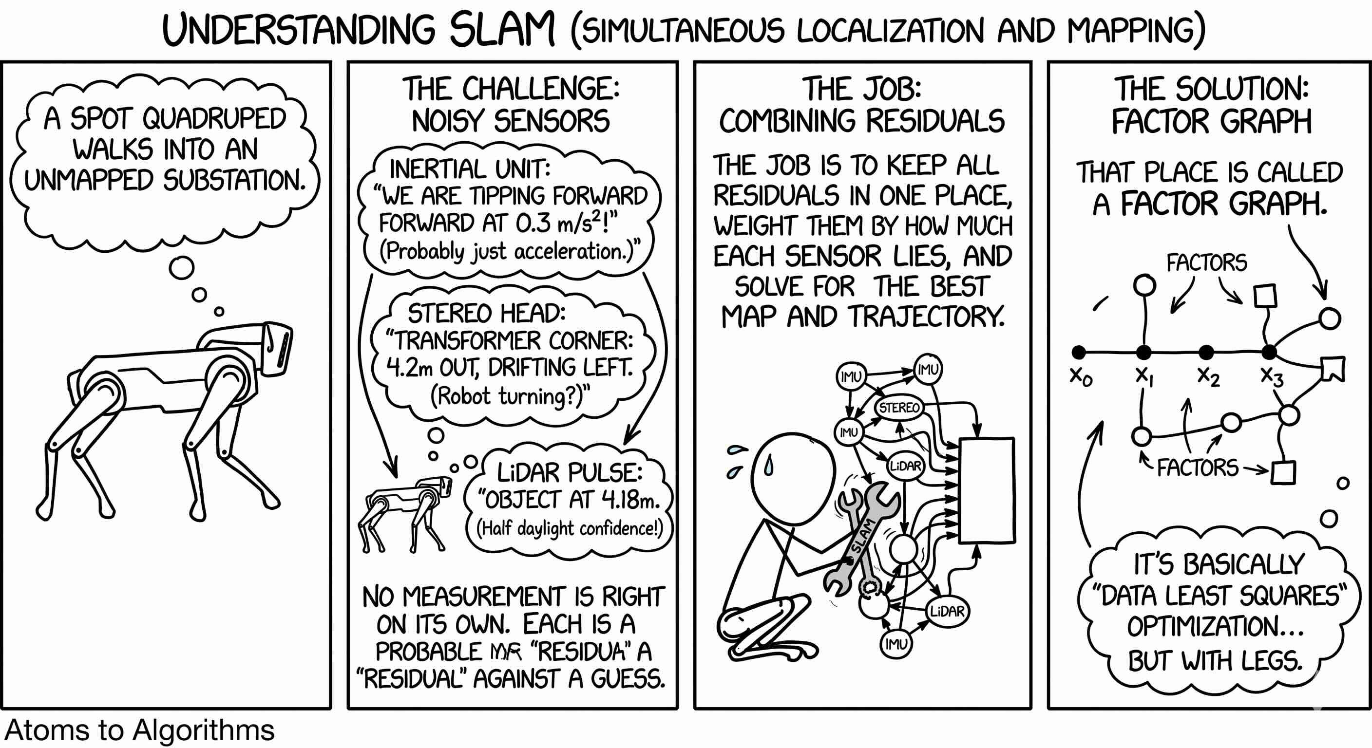
A Spot quadruped walks into an unmapped substation. Its inertial unit says it is tipping forward at 0.3 m/s². The stereo head says the corner of the nearest transformer is 4.2 meters out and drifting left as the robot turns. A LiDAR pulse comes back at 4.18 meters, with half the confidence that daylight gave it outdoors. No measurement is right on its own. Each one is a residual against the robot’s best current guess of where it stands. The whole job of SLAM (Simultaneous Localization and Mapping) is to keep all the residuals in one place, weight them by how much each sensor lies, and solve for the trajectory and the map that make the residuals as small as possible. That place is called a factor graph.
In last post we put a camera inside a robot’s fingertip. Today we lift the sensor out of the finger and ask the larger question that has organized robotics perception for the last fifteen years. A robot walks into a place it has never been, with sensors that disagree with each other. How does it figure out where it is, build the map as it moves, and snap the map back into consistency when it returns somewhere it has been before? The same answer drives Amazon’s warehouse fleet, Boston Dynamics’ Atlas, and the Roomba in your living room: a factor graph, with a loop closure that lives inside it. In a way you can think of how tesla FSD works, as it can go on uncharted roads as well
How it actually works
Picture the robot’s life as a string of beads. Each bead is a pose: where the robot was at one moment, in three-dimensional space. Some beads are the robot itself; others are landmarks it has seen, like the corner of that transformer. Between every two beads runs a piece of string, a constraint that says these two beads should be a certain distance apart, in a certain orientation, with a certain confidence. A camera measurement is a string. An inertial measurement is a string. A GPS fix is a string. Wheel odometry is a string.
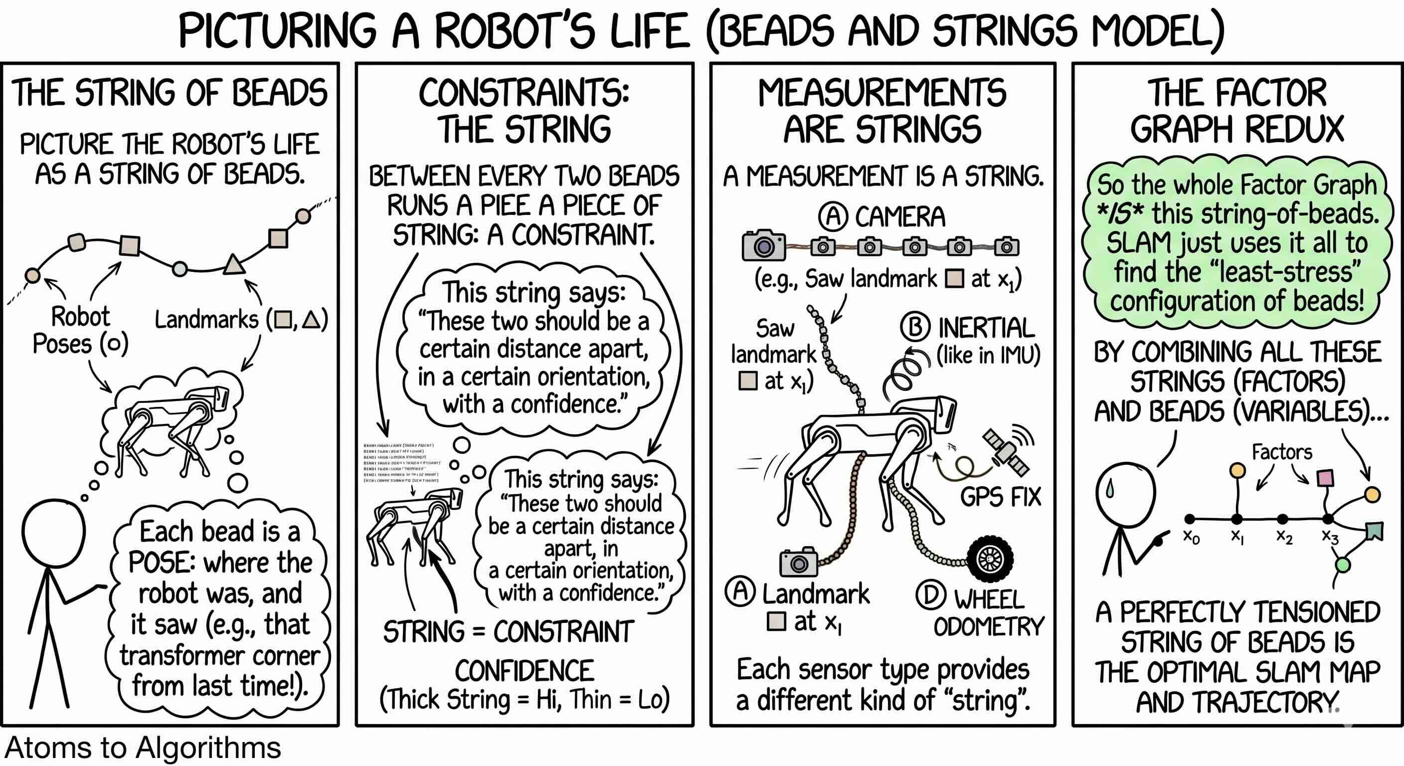
The collection of beads and strings is a graph. In the field’s language it is called a factor graph, with beads as variables and strings as factors. Some strings are short and stiff (a high-confidence stereo measurement of a feature one meter away). Others are long and stretchy (an odometry estimate integrated across two seconds of walking). The optimizer wiggles the beads in space until the strings are as relaxed as possible, with the stiff ones honored more than the stretchy ones. That trust-weighting is the whole secret. Came across this interesting paper explaining around it.
The deep insight, due to Frank Dellaert at Georgia Tech and the GTSAM library his group built, is that this wiggle does not have to start from scratch each time a new measurement arrives. The factor graph can be reorganized into a tree where new measurements only disturb a small part of it. Michael Kaess and coauthors made this incremental in 2012 with a paper called iSAM2, and almost every modern SLAM system runs some version of that algorithm under the hood.
Loop closure is where the math earns its keep. A robot drives a square around a building. After thirty seconds it has accumulated drift; its trajectory thinks it is back at the starting hallway but actually it is three meters off, because every odometry measurement is a tiny lie that compounds. Then a place-recognition module notices that the current view matches one from a thousand frames ago. The system adds a factor connecting the current pose to that old pose. The optimizer back-propagates the new constraint through every pose in between. The whole trajectory snaps back into consistency. That is the difference between visual odometry, which drifts forever, and SLAM, which closes the loop. The point is small error compounds and you have to be mindful of it.
The 2026 wave is foundation models eating the front of the SLAM pipeline. Two weeks ago we watched FoundationStereo collapse stereo depth into a single learned forward pass. This week, two new papers (FoundationSLAM in December, Keep It CALM in April) push the same logic further: a calibration-free, learned visual frontend that produces depth, motion, and pose hypotheses, paired with a small classical backend that still runs the factor graph because the math underneath it has not been improved on. The Gaussian-splatting wave (VIGS-SLAM and friends) replaces the implicit 3D map with millions of differentiable colored splats. The factor graph stays.
New this week
A team in April released SNGR, a system that wraps iSAM2 with a clever sampler for the cases where the standard Gaussian-shaped trust assumptions fail (range-only SLAM, ambiguous matches). It is the first paper in years that treats the failure modes of the standard pipeline as the central problem rather than the corner case.
Amazon Science published a method for what they call “lighthouses”: active SLAM for low-compute, narrow-field-of-view robots, the kind that ship into homes rather than warehouses. It is a quieter result but a more honest one: most consumer robotics has one tenth of the compute budget that a humanoid program has, and the math has to bend accordingly. Which makes me wonder if there will be two different types of companies - consumer humanoid and enterprise serving robotics.
VIGS-SLAM, a December 2025 paper, tightly couples a stereo and inertial frontend with a 3D Gaussian Splatting map, jointly optimizing camera poses, depths, and inertial states in one graph. The clearest current evidence that the splatting-versus-mesh debate has tipped toward splats for online SLAM.
What to notice
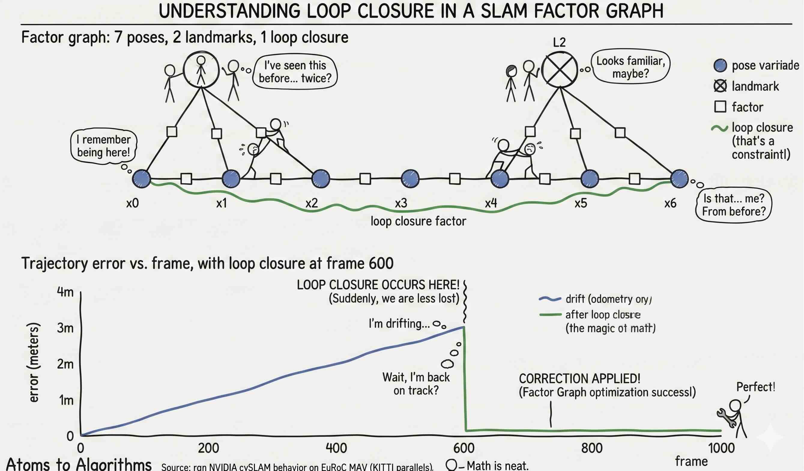
The visualization is a two-panel sketch. The top panel is a small factor graph: poses along a trajectory drawn as circles, landmarks as larger circles, factors as squares on the edges, with the loop-closure factor connecting the last pose back to the first drawn with a thicker outline. The bottom panel shows trajectory error growing linearly across six hundred frames of pure odometry, then snapping flat the moment the loop closes. The takeaway: one loop-closure factor does not adjust one pose; it back-propagates through every pose in between. A long, slow drift collapses to almost nothing the instant the robot realizes it has been somewhere before.
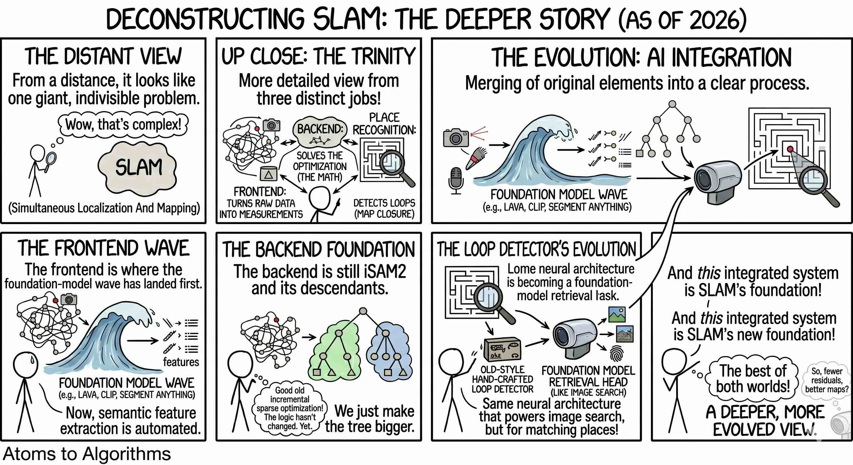
The deeper story is that SLAM looks like one problem from a distance and like three up close: a frontend that turns raw sensor data into measurements, a backend that solves the optimization, and a place-recognition layer that detects loops. The frontend is where the foundation-model wave has landed first. The backend is still iSAM2 and its descendants. The place-recognition layer is becoming a foundation-model retrieval head, the same neural architecture that powers image search.
Tomorrow we look at the trick that lets all of this run on a robot moving at human speed: IMU pre-integration. A thousand inertial samples per second cannot be added to the factor graph one at a time without melting the optimizer. The trick is a piece of math from 2012, refined in 2017, that compresses a whole burst of inertial samples into a single factor in the graph at ten samples per second, with a closed-form way to update the answer when the optimizer changes its mind about the sensor’s bias. It is the most-cited mechanism in modern visual-inertial odometry and the reason a Unitree G1 or an electric Atlas can stride at 1.5 meters per second and still keep its head straight on the map.
Subscribe for tomorrow’s read. We’re walking the robotics supply chain from atoms to algorithms, one weekday at a time.
Sources: